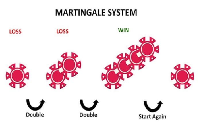
The martingale strategy is often presented as a simple progression: start with a small stake, double it after every loss, and return to the original amount after a win. On paper, the attraction is obvious. A single winning bet can recover the previous sequence of losses and leave a small profit.
The problem is what happens before that win arrives.
A martingale strategy does not change the probability of the underlying game. It changes how much money is committed when the player is already experiencing a losing sequence. That distinction is the key to understanding both its appeal and its risk.
How The Martingale Strategy Actually Progresses
The classic martingale strategy begins with a fixed base stake. After a loss, the next stake is doubled. After a win, the progression resets to the original stake.
For example, with a starting stake of one unit:
1 → 2 → 4 → 8 → 16 → 32 → 64 → 128
If the 1-unit bet loses, the next bet becomes 2 units. If that also loses, the stake becomes 4 units.
The progression continues until a win occurs or the player reaches a bankroll or table limit.
The important detail is that the system does not require the next win to be unusually large. On a standard even-money bet, a 16-unit winning stake produces 16 units of profit. That can recover the previous 15 units lost through the 1, 2, 4 and 8-unit bets and leave a 1-unit gain.
That is the mathematical feature that makes the martingale strategy look attractive during short sequences.
The Numbers Reveal The Real Problem
Consider what happens after consecutive losses:
| Consecutive Losses | Next Stake From 1 Unit | Total Already Staked |
| 1 | 2 | 1 |
| 2 | 4 | 3 |
| 3 | 8 | 7 |
| 4 | 16 | 15 |
| 5 | 32 | 31 |
| 6 | 64 | 63 |
| 7 | 128 | 127 |
| 8 | 256 | 255 |
After eight consecutive losses, the next required stake is 256 units, while 255 units have already been committed.
The progression has therefore transformed a 1-unit starting bet into a requirement for another 256 units.
This is the central weakness of the martingale strategy. The original stake may look insignificant, but the later exposure can become enormous.
Why One Winning Bet Looks So Convincing
Suppose the sequence is:
1 → 2 → 4 → 8 → 16
The first four bets lose and the fifth wins.
The calculation is:
- First loss: −1
- Second loss: −2
- Third loss: −4
- Fourth loss: −8
- Total losses: −15
- Fifth bet wins: +16
Final result:
+1 unit
This is the most persuasive part of the martingale strategy.
A player can experience several consecutive losses and then see one winning round apparently repair the entire sequence.
But consider what happens if the 16-unit bet also loses.
The accumulated loss becomes:
1 + 2 + 4 + 8 + 16 = 31 units
The next required stake is now 32 units.
The strategy hasn’t become more likely to succeed. The amount at risk has simply increased.
A Small Starting Stake Does Not Mean Small Risk
This is one of the most common misunderstandings surrounding the martingale strategy.
A player might think:
“I’m only starting with one unit, so the risk is tiny.”
That describes the first bet, not the complete progression.
With a 1-unit base stake:
- Five consecutive losses require 31 units in total.
- Six require 63 units.
- Seven require 127 units.
- Eight require 255 units.
- Ten require 1,023 units.
The relationship is exponential.
The next required stake after ten losses is 1,024 units.
Therefore, the relevant question isn’t simply how much the first bet costs. It is how much capital is available if the losing sequence continues.
A 100-Unit Bankroll Shows The Constraint Clearly
Imagine a hypothetical player with 100 units and a 1-unit starting stake.
The progression can reach:
1 → 2 → 4 → 8 → 16 → 32 → 64
The total exposure after seven consecutive losses would be 127 units, which exceeds the available 100-unit bankroll.
So the player cannot complete the theoretical progression.
The martingale strategy therefore encounters a practical limit before the mathematical sequence itself reaches infinity.
This is why bankroll size must be considered alongside the starting stake.
Table Limits Create Another Barrier
Bankroll isn’t the only constraint.
Casinos impose maximum bet limits, and those limits can interrupt the progression even when the player has sufficient money.
For example, consider a table with a 100-unit maximum bet and a 1-unit starting stake.
The progression is:
1 → 2 → 4 → 8 → 16 → 32 → 64
After losing 64 units, the next theoretical stake is 128 units.
But the table allows only 100.
The player can no longer follow the standard progression.
A martingale strategy therefore depends on two finite resources: available bankroll and permitted maximum stake.
Neither can be assumed to be unlimited.
European Roulette Makes The Probability Easy To See
European roulette provides a useful mathematical example because the probabilities are straightforward.
Suppose the bet is Red or Black.
There are:
- 18 red numbers
- 18 black numbers
- 1 zero
- 37 total pockets
The probability of winning a Red/Black bet is:
18/37 ≈ 48.65%
The probability of losing is:
19/37 ≈ 51.35%
The zero is neither red nor black, so it contributes to the losing side of the wager.
The standard house edge on this even-money bet is approximately 2.70%.
The martingale strategy does not remove that edge.
It simply changes how the stakes are distributed across successive bets.
Losing Streaks Are The Real Stress Test
If the probability of losing one Red/Black bet is approximately 0.5135, the probability of experiencing n consecutive losses from a specified starting point is:
0.5135ⁿ
That gives approximately:
| Losing Streak | Probability |
| 3 losses | 13.54% |
| 5 losses | 3.57% |
| 6 losses | 1.83% |
| 8 losses | 0.48% |
| 10 losses | 0.13% |
A ten-loss sequence is considerably less common than a three-loss sequence.
But “unlikely on one particular sequence” should not be confused with “impossible during repeated play.”
The more rounds someone plays, the more opportunities exist for unusual sequences to occur.
That is particularly relevant to the martingale strategy, because its largest financial exposure occurs precisely when a long losing sequence develops.
Session Length Changes The Risk Picture
Consider sessions of:
- 20 rounds
- 50 rounds
- 100 rounds
- 200 rounds
The probability of a particular ten-loss sequence remains the same when viewed from one specific starting point.
But over a long session, there are many potential places where a losing run could begin.
This creates an important difference between:
“What is the probability of ten losses beginning on this particular round?”
and:
“What is the probability of encountering a ten-loss sequence somewhere during a long session?”
Those are not the same question.
For anyone examining a martingale strategy, this distinction matters because repeated opportunities can make rare sequences increasingly relevant.
The Next Outcome Is Not “Due”
Another major problem is gambler’s fallacy.
Suppose a roulette sequence produces:
Red → Red → Red → Red → Red
It is tempting to think Black is now more likely.
It isn’t.
On the next independent spin, the probabilities remain:
- Red: 18/37
- Black: 18/37
- Zero: 1/37
The previous results do not create a debt that the wheel has to repay.
This is particularly important after a losing sequence under the martingale strategy. A player may feel that the next wager has become more attractive because several previous bets failed.
The probability hasn’t changed.
The stake has.
The Martingale Strategy Changes Exposure, Not Probability
This distinction is the foundation of the entire subject.
Imagine two players making the same Red/Black bets.
Player A uses flat staking:
1 → 1 → 1 → 1 → 1
Player B uses a martingale strategy:
1 → 2 → 4 → 8 → 16
The roulette wheel doesn’t know which staking system is being used.
The probability of the next outcome is identical for both players.
The difference is how much money Player B has exposed after previous losses.
That means progressive staking cannot turn a negative-expectation game into a positive-expectation one.
Martingale Strategy Vs Flat Staking
| Feature | Flat Staking | Martingale Strategy |
| Base stake | Fixed | Fixed initially |
| After a loss | Same stake | Doubles |
| After a win | Same stake | Usually resets |
| Exposure during losing streak | Relatively stable | Rises rapidly |
| Underlying probability | Unchanged | Unchanged |
| House edge | Unchanged | Unchanged |
| Bankroll pressure | More predictable | Can escalate sharply |
| Table-limit sensitivity | Lower | High |
Flat staking doesn’t make the underlying game favourable either.
Its main difference is that losing streaks don’t automatically force the next wager to become dramatically larger.
With the martingale strategy, the player’s financial exposure becomes concentrated toward the point where the losing sequence is already at its longest.
Why Frequent Small Recoveries Can Be Misleading
Imagine someone repeatedly experiences this pattern:
Loss → Loss → Win → Reset
The account may show many small successful recoveries.
That can create the impression that the martingale strategy is consistently working.
But a strategy shouldn’t be judged solely by how often it produces a small positive session result.
The size of the occasional loss matters.
If many sessions produce +1 unit but one prolonged losing sequence produces −127, −255 or −1,023 units, the frequency of small wins can create a misleading picture of sustainability.
This is one reason looking only at the percentage of winning sessions is insufficient.
Bankroll And Table Limits Are Part Of The Strategy
A theoretical progression can continue indefinitely on paper.
Real play cannot.
A player may encounter:
- Insufficient bankroll
- Maximum table stake
- Maximum platform stake
- Personal session limit
- Withdrawal or deposit constraints
- A decision to stop after reaching a predefined loss
Once the required next stake cannot be placed, the standard recovery mechanism no longer works.
The martingale strategy therefore has a built-in practical dependency on financial limits.
Those limits aren’t minor details. They determine how far the progression can actually go.
What Happens When The Progression Breaks?
Suppose someone has a 100-unit bankroll and starts at one unit.
After six losses:
1 + 2 + 4 + 8 + 16 + 32 = 63 units
The next required stake is 64.
If that loses too, the player has lost 127 units in total—more than the original bankroll.
So the player cannot complete the theoretical recovery sequence.
The attractive idea of “one eventual win recovers everything” has a hidden condition:
The eventual win must arrive before the player is unable to continue the progression.
That condition is precisely where bankroll and table limits become important.
A Platform Should Be Evaluated Separately From The Staking System
The martingale strategy is a mathematical staking concept; the platform where someone plays is a separate question.
Before starting a session, players should understand the applicable game rules, minimum and maximum stakes, transaction conditions and responsible-play tools rather than assuming that a particular staking progression changes the game’s mathematics.
For readers evaluating the wider platform environment, Nagad88 can be considered separately from the analysis of the staking method itself.
The same principle applies regardless of platform: the rules of the underlying game determine its probabilities, while the staking system determines how much is placed at risk.
Session Limits Matter More Than The Starting Number
A useful practical safeguard is to decide the session parameters before beginning rather than changing them after losses.
That means defining:
- Starting bankroll
- Base stake
- Maximum acceptable loss
- Maximum number of progression steps
- Maximum session duration
- Point at which play stops
A martingale strategy becomes particularly difficult to control when the player keeps increasing the permitted exposure simply because the previous progression failed.
A predefined stopping point prevents the next required stake from becoming an emotional decision.
Other Staking Systems Do Not Change The Underlying Game
Martingale is not the only staking progression.
Flat Staking
The same amount is wagered each round.
D’Alembert
The stake generally increases by one unit after a loss and decreases after a win.
Fibonacci
The stake follows a Fibonacci-style sequence rather than doubling immediately.
Reverse Martingale
The stake increases following wins rather than losses.
Fixed-Percentage Staking
The wager is calculated as a percentage of the available bankroll.
These approaches behave differently in terms of exposure, but none changes the probability generated by an independent random game.
That is the important distinction between staking mechanics and game mathematics in Nagad88.net.
A Better Way To Judge The Martingale Strategy
Instead of asking simply, “Does Martingale work?”, look at the entire risk structure.
Ask:
- What is the underlying game’s probability?
- What is its house edge?
- What is the starting stake?
- How much bankroll is available?
- What happens after five consecutive losses?
- What happens after eight?
- What is the table maximum?
- How many rounds might the session contain?
- What is the maximum planned exposure?
- What happens when the progression can no longer continue?
Those questions reveal substantially more than looking at the number of winning sessions.
The Real Lesson Behind Progressive Staking
The appeal of the martingale strategy comes from a genuine mathematical feature: on an even-money bet, a sufficiently large winning stake can recover the preceding losses and produce the original one-unit profit.
But the same mathematics creates the problem.
Every additional loss requires another doubling.
1 → 2 → 4 → 8 → 16 → 32 → 64 → 128 → 256
The system therefore converts a small initial exposure into increasingly large financial requirements.
The underlying game hasn’t become more favourable.
The next outcome hasn’t become more predictable.
The losing sequence hasn’t made a win “due.”
Only the amount being wagered has changed.
Final Takeaway: The Stake Is Growing, Not The Probability
The martingale strategy is best understood as a progressive staking system rather than a method for predicting random outcomes.
Its apparent strength is easy to demonstrate: a single win can recover a sequence of previous losses when the required stake can still be placed.
Its weakness is equally clear: the amount required to reach that recovery point grows exponentially.
A 1-unit starting stake can eventually require 256 units after eight losses and 1,024 units after ten. A finite bankroll or table maximum can stop the progression before the desired recovery win arrives.
For readers studying the martingale strategy, the most important question is therefore not whether a winning round can recover previous losses. It can.
The more useful question is how much exposure is required to reach that winning round, and what happens if the losing sequence lasts longer than the available bankroll allows?
That is where the mathematics of progressive staking becomes much more important than its simple 1-2-4-8 appearance.